Deconvolution

The simplest way to describe a convolution is a blur: a single pixel becomes a blur. If you move your camera while taking a picture, a point will become a sweep, and a line will become an area. It is easy to create a blur like this via software. It is harder to remove them, and that is what devonvolution is about.

The deconvolution described here is via Fourier transformation (see other article on my Math Page).

Deconvolution via Fourier

Convolution, h is the convoluted function, g is the original, and f is the "blur" function

In case there is no "blur" f is the Dirac Delta function:

Fourier transformation of function f and h:

Here the discrete Fourier analysis is used and the limits of the convolution need to be taken modulo 2π:

Now the opposite operation, deconvolution. In the following the input functions are denoted as fa(x,y), fb(x,y), fh(x,y) as they apply to pictures (x, and y coordinate) and the Fourier transform of these functions as Fa(fx, fy), Fb(fx, fy),  Fh(fx, fy), as they give the amplitude and phase of frequencies fx, fy.

Given a function fb which is function fa convoluted via fg, what would the original fa be? For this we also need to know what the same convolution does to a example function: fh is ff convoluted by the same fg:

And with Fa given (=Fourier transform from function fa) function fa can be calculated. So within reason, a given convolution can be undone.

The previous formulae written in words means:

Suppose the same convolution has blurred many pictures, then one example of which you have the convoluted (say blurred) version and the clear version will be sufficient to unblur the rest.

Already a few remarks can be made about it:

· The quotient shows that zero in the nominator or denominator will give trouble

· The convolution (blur function) of both pictures must be the same

· In this example the blur is modulo the size of the picture, e.g. if affects a pixel size_x+2 this will become 2. If you don't do this you will lose information and around the borders the deconvolution does a poor job.

· In deconvolution details matter, and the 8 bit per colour used in BMP files is good enough for a deconvolution, but JPEG is not. It is a lossy data compression technique that in general loses too much information.

· The formulae as shown requires three Fourier transformations, and one reverse Fourier transformation. On pictures these are all lengthy operations.

To start with the last problem: the many lengthy operations needed. When dealing with one type of convolution one could store the quotient  in a file, saving you at least two Fourier transforms.

But there is a way to avoid any forward and reverse Fourier transform of the file that is to be deconvoluted. For this you use the fact that both operations are linear, and you can Fourier transform a single pixel, apply the quotient and transform this back. Now one pixel is transformed into a whole picture. The next pixel is that picture shifted, and multiplied by the colour of the next pixel.

In the program here, this file that contains that pixel deconvoluted is called a stamp file (extension .stp). If the deconvolution is simple, most values in this file are zero and there is some analysis to check if this is the case, and to see if the "stamp" size can be reduced.

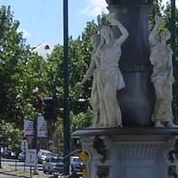
Example Single pixel (Clear picture) F	Clear Picture A
Example Single pixel, blurred H	Blurred picture B

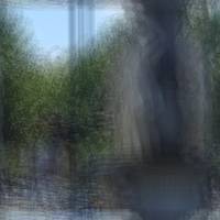
When pictures F, H, and B are given A can be calculated, when the blur operation that affected F and A are the same.

Use of the deconvolution program

The deconvolution program must calculate the Fourier transformation and reverse in some case (depending on operations chosen) and this is a time consuming operation. The time needed increases with the square of the area (length times height). So when one doubles the size of a picture, the area becomes 4 times bigger and the time needed for a Fourier transform becomes sixteen times more. So try small pictures (say 200 x 200) first. There is a dialog that enables you to choose a blur. Use the same blur for both the example and the picture. Once you have "blurred" and saved the example and the picture, you are ready for the deconvolution. The deconvolution dialog allows you to choose the "Clear Example" file, the "blurred Example" file and the blurred picture file. It will save the Fourier transformation as an .ft file on your disk, so allow this program some diskspace.

The "Deconvolute File" item is under the "Blur" menu item. Here the "Example Files" can be chosen. You can also test the result, by entering the filename of the original file.

Compare Result

There is a compare function built in, under the "Blur" menu item. The filename of the original file can be entered via the "Deconvolute File" item which is also under the "Blur" menu item. The result will show a 20 times amplification of the difference between the two pictures. The main reason for the difference is the 8 bit resolution of a colour per pixel. Heavily blurred pictures will give a poorer result because of this. But also in the very white area's the quality will be limited, because of the 255 maximum value available.

Download Deconvolute.exe